Using DuckDB to analyze over 95 million taxi rides

Hi, this is Gregor, head of the Data Visualization team at Datawrapper. This week I tried using DuckDB to prepare a massive dataset for a Datawrapper map.

Tools like Datawrapper try to make it easy to visualize a dataset. Charts, tables, and even interactive maps can be created in no time — if you have a fitting dataset!

But what if your data comes in a format or size that you can’t just throw into Datawrapper? So, as a challenge for this week, I wanted to look at a massive dataset and found one for over 95 million taxi rides in New York City in 2023.

So before I go into how I analyzed the data, here’s the first map I created.

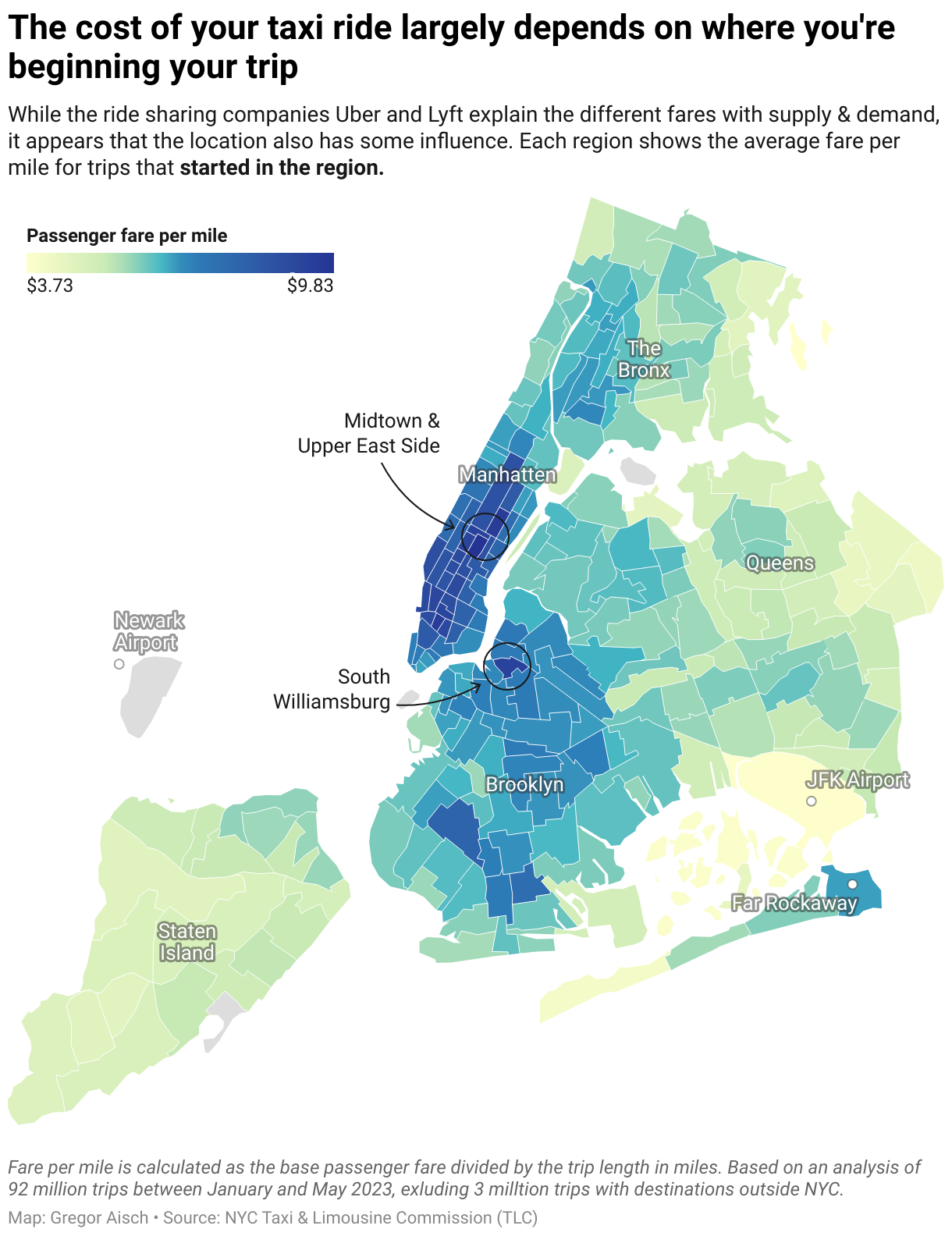
The data for the map is published by the NYC Taxi & Limousine Commission (TLC) and comes as Parquet files, each of which stores taxi rides for one month. They publish separate files for “yellow” and “green” taxis, but for this blog post, I picked the biggest dataset which is about the “for-hire vehicles” aka. Uber and Lyft.

What is DuckDB, and why use it?

Usually, I would write a script in some data analysis framework, like R or Python Pandas. But I wanted to try a more traditional approach to analyzing the data. Back in university, I learned that there are programs for managing and analyzing large datasets, and they are called databases^[1]. Yet, I’ve rarely encountered or used databases in over ten years of doing data journalism.

One thing that’s great about databases is that you can write your analysis queries in a language called SQL (Structured Query Language) that almost reads like English sentences, like this one, for example:

SELECT name FROM employees WHERE birthday = TODAY()

The reason that working with databases such as MySQL or PostgreSQL can be cumbersome is that there’s a lot of setup work to install a database server on your computer, and often it’s not trivial to understand where the data is actually stored. Also loading and exporting data from various formats is not trivial. And that’s where DuckDB comes in!

It’s a relatively new database designed for exactly this task: analyzing datasets that are too big to handle in Excel but still small enough to fit in your computer’s memory. You can use DuckDB on the command line, but also inside many tools and frameworks (like DBeaver or R – it even runs directly in web browsers).

So let’s move on to importing the taxi ride dataset into DuckDB.

Reading and analyzing the data

The first step is downloading the Parquet files to your computer and loading them into a DuckDB database. Before doing so, let’s take a look what variables are included in the tables.

The TLC publishes a data dictionary that explains all the available columns. There is a lot more interesting information in the data (exact time of the trips, tips paid to the driver, passenger counts), but for this analysis, we’ll just look at these columns:

Field	Explanation
hvfhs_license_num	The TLC license number of the HVFHS base or business
PULocationID	TLC Taxi Zone in which the trip began
DOLocationID	TLC Taxi Zone in which the trip ended
trip_miles	Total miles for passenger trip
base_passenger_fare	Base passenger fare before tolls, tips, taxes, and fees

I used the following query to read the files. Note that DuckDB automatically recognizes the file extension .parquet and knows to use the read_parquet function. The wildcard * in the query told DuckDB to conveniently read all the matching Parquet files in the current directory into one table.

CREATE TABLE rides AS SELECT 
	hvfhs_license_num,
	PULocationID,
	DOLocationID, 
	base_passenger_fare,
	trip_miles
FROM './fhvhv_*.parquet';

This took about 5-6 seconds to run, and now I have a table rides with over 95 million rows ^[2].

Now we want to group the taxi rides by pickup zone (the city region where the trip started) and calculate the fare per mile by dividing the fare by the trip distance. Note that the query excludes rides with an unknown drop-off zone (which I assume are rides ending outside New York City).

SELECT 
    PULocationID pickup_zone,
    AVG(base_passenger_fare / trip_miles) fare_per_mile,
    COUNT(*) num_rides 
FROM rides 
WHERE DOLocationID < 264 
GROUP BY PULocationID;

With my data already loaded into memory, the above query took about 100 milliseconds! Before exporting the data to CSV, I wanted to exclude the numbers for pickup zones where the sample is too small (less than 100 rides). One way SQL lets you do this is to nest queries inside other queries. In the inner query, we’re counting the rides for each pickup zone and storing the result as num_rides, and in the outer query, we’re setting the fare_per_mile to NULL for all zones where we have fewer than 100 rides:

SELECT 
    PULocationID pickup_zone,
    "Zone",
    IF(num_rides >= 100, fare_per_mile, NULL) fare_per_mile,
    num_rides
FROM (
    SELECT
        PULocationID, 
        AVG(base_passenger_fare/trip_miles) fare_per_mile, 
        COUNT(*) num_rides
    FROM rides 
    WHERE DOLocationID < 264 GROUP BY PULocationID
)

One more thing I needed to do was to merge the resulting table with the names of the pickup zones. The TLC publishes a separate table with the names of the taxi zones, and thanks to DuckDB, we can simply address it by throwing in the URL of the CSV file! The final query I used for the map above is this:

COPY (
    SELECT 
        PULocationID pickup_zone,
        "Zone",
        IF(num_rides >= 100, fare_per_mile, NULL) fare_per_mile,
        num_rides
    FROM (
        SELECT
            PULocationID, 
            AVG(base_passenger_fare/trip_miles) fare_per_mile, 
            COUNT(*) num_rides
        FROM rides 
        WHERE DOLocationID < 264 GROUP BY PULocationID
    ) rides JOIN (
        SELECT LocationId, "Zone"
        FROM 'https://d37ci6vzurychx.cloudfront.net/misc/taxi+_zone_lookup.csv'
    ) zones ON (LocationId = PULocationID)
) TO './output.csv' (HEADER, DELIMITER ',');

Et voila, that’s the data we can throw into Datawrapper, along with a custom basemap for the Taxi zones. To create the basemap, I downloaded the Shapefile from the TLC website and converted it to TopoJSON in Mapshaper (here’s a handy tutorial if you’ve never done this before).

Let’s dive in some more.

If you got this far, we might as well dig a little deeper. Since the hvfhs_license_num field in the data tells us which ride-sharing company provided the service, we can compare the fare per mile for Uber and Lyft. In the next query we’re simply computing the average fare per mile for each service provider:

SELECT 
   hvfhs_license_num,
   AVG(base_passenger_fare/trip_miles) fare, 
   COUNT(*) 
FROM rides GROUP BY hvfhs_license_num;

hvfhs_license_num	fare	COUNT(*)
HV0005 (=Lyft)	6.23	26,155,420
HV0003 (=Uber)	7.01	69,690,700

So as we see, the average fare for Lyft rides is $6.23 per mile, while the average Uber ride costs $7 per mile. We can also tweak the query a little bit to run the above regional analysis for each provider separately:

-- Uber rides
CREATE TABLE uber_rides AS SELECT 
    PULocationID,
    AVG(base_passenger_fare/trip_miles) fpm_uber,
    COUNT(*) cnt_uber
FROM rides 
WHERE hvfhs_license_num = 'HV0003' AND DOLocationID < 264
GROUP BY PULocationID

-- Lyft rides
CREATE TABLE lyft_rides AS SELECT 
    PULocationID,
    AVG(base_passenger_fare/trip_miles) fpm_lyft,
    COUNT(*) cnt_lyft
FROM rides 
WHERE hvfhs_license_num = 'HV0005' AND DOLocationID < 264
GROUP BY PULocationID;

Now all that’s left to do is to join both queries and calculate the differences between the average Uber fare per mile and the average Lyft fare per mile for each taxi district, but only if we have at least 100 rides from each company:

SELECT 
    rides_uber.PULocationID pickup_zone,
    cnt_uber,
    cnt_lyft,
    IF(cnt_uber >= 100 AND cnt_lyft >= 100, fpm_uber - fpm_lyft, NULL)
FROM uber_rides
JOIN lyft_rides ON (uber_rides.PULocationID = lyft_rides.PULocationID)

Which brings us to the final map of this blog post:

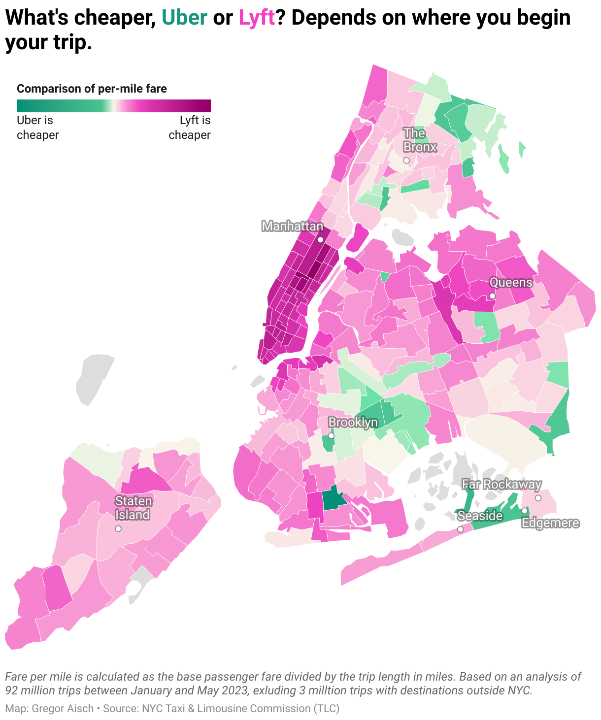
The map confirms that Lyft is generally the cheaper option, except for some remote areas where Uber is cheaper. Of course, that also means that Lyft pays its drivers less – but if you care about that, you probably shouldn’t use Uber or Lyft and just order a regular taxi.

I hope you enjoyed this little excursion into the world of databases and huge data sets. We’ll see you next week!

1. Technically, the term database management system (DBMS) is more precise. ↩︎
2. Parquet is a column-based data format, which means that it’s a lot faster to read only a few columns instead of the whole table – as opposed to a row-based format like CSV. ↩︎