How to calculate shaded relief for the entire world with GDAL, fast

Hi everyone, this is Anna – I’m working on keeping administrative regions in the Datawrapper choropleth and symbol maps up to date (e.g. districts, ZIP code areas, states …). I’m also responsible for the shaded relief in our locator maps.

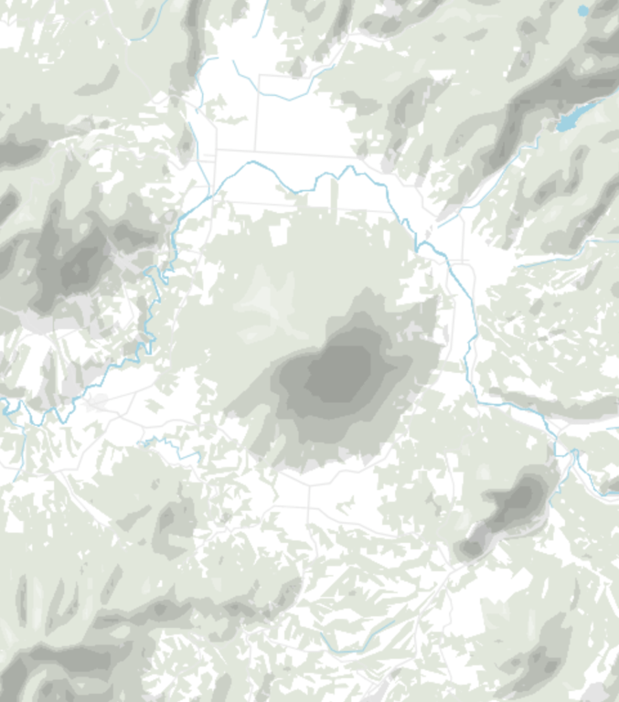
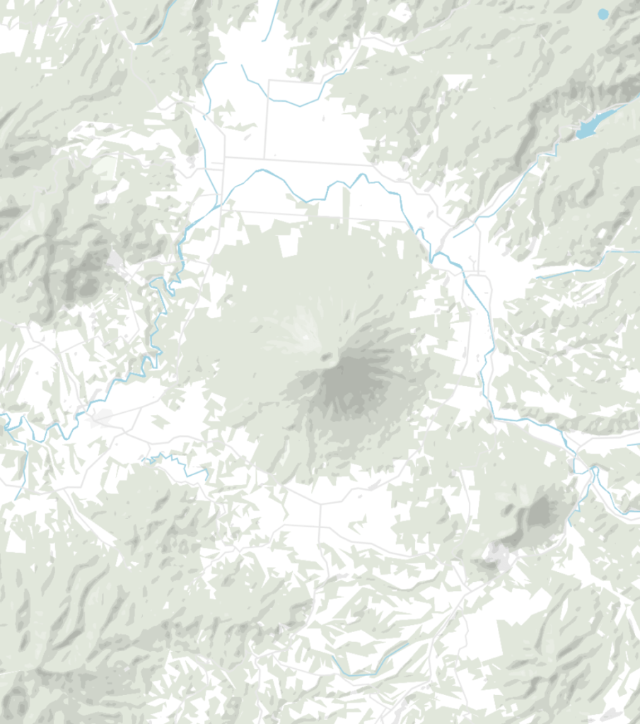
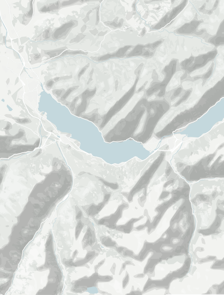
Shaded relief (what we call the “Mountains” feature in our locator maps) has been a feature in Datawrapper since November 2019. Recently, we improved the quality: Our mountains now look crisper with a higher resolution, going all the way to zoom level 10.

To try it out yourself, create a new locator map here (no need to sign in or up), then go to step 2: Design Map and select “Mountains”.

• 

• 

The following article is a technical, high-level walkthrough on how we generated shaded relief for the entire world with NASA data and the help of GDAL, a library for processing geodata. We won’t go into much detail how to download the data, set GDAL up, etc., but we will name and explain some formulas. Let’s start!

Shaded relief: What is is

Shaded relief – also called “hillshading”, “hill shading” or, more broadly, “terrain” – is a technique to indicate shapes of mountains on a map. Two-dimensional topographic information is important for navigation and accurately representing the landscape. But shaded relief is not an exact measure of heights or true representation of mountains, but rather hints how steep the terrain is.

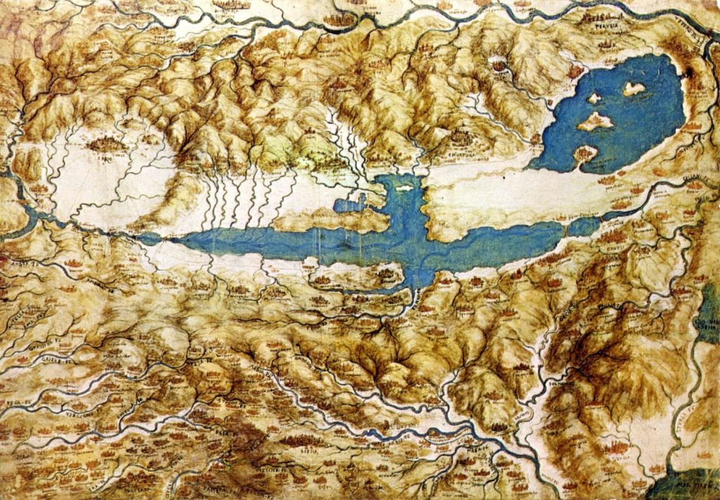
An early example of visualizing mountains can be seen in one of Leonardo da Vinci’s map of Tuscany from 1503, where the mountains are sketched as small hills:

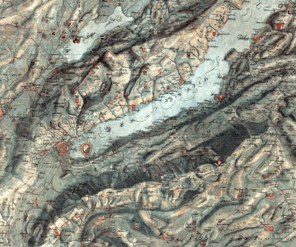
One of the first known use of shaded relief in cartography was by Swiss cartographer Hans Conrad Gyger in 1668. He created a military map with shaded relief as we know it today: a visual 3D effect of the topography, created by an artificial light source:

Today, shaded reliefs are standard practice. There are numerous ways to generate shaded reliefs for digital maps: Desktop apps like QGIS have a shaded relief function, 3D graphics tools like Blender can be used to generate shaded relief, and it can be calculated directly in the browser.

At Datawrapper, the decision on how to create our shaded relief was driven by our users: We wanted to enable them to edit the shaded relief – like the rest of their locator map – in vector graphics software like Adobe Illustrator after they download it as PDFs or SVGs. So we decided to implement shaded relief as a vector tile layer. Let’s see how we went about this:

1. Getting DEM data from NASA

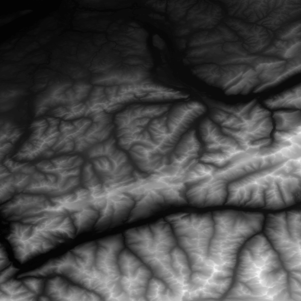
To be able to calculate shaded relief, we needed elevation data. One common format is the Digital Elevation Model (DEM). In a DEM, the elevation data is stored in the pixels of a raster – each pixel has a certain gray value, which represents a height value.

For this project, we decided to use the ASTER DEM.^[1]The data covers the entire world up to ±80° latitude and comes in 22,192 TIFFs with a total size of 380GB. Each TIFF shows 1° by 1° (approximately 30 meters at the equator):

To process the DEM, we used three tools:

• GDAL, a translator library for raster and vector geospatial data formats
• Python, a programming language
• PostGIS, an extension for PostgreSQL that can handle geographical objects and functions. We used it to store the shaded relief vectors.

2. Calculating shaded relief with GDAL

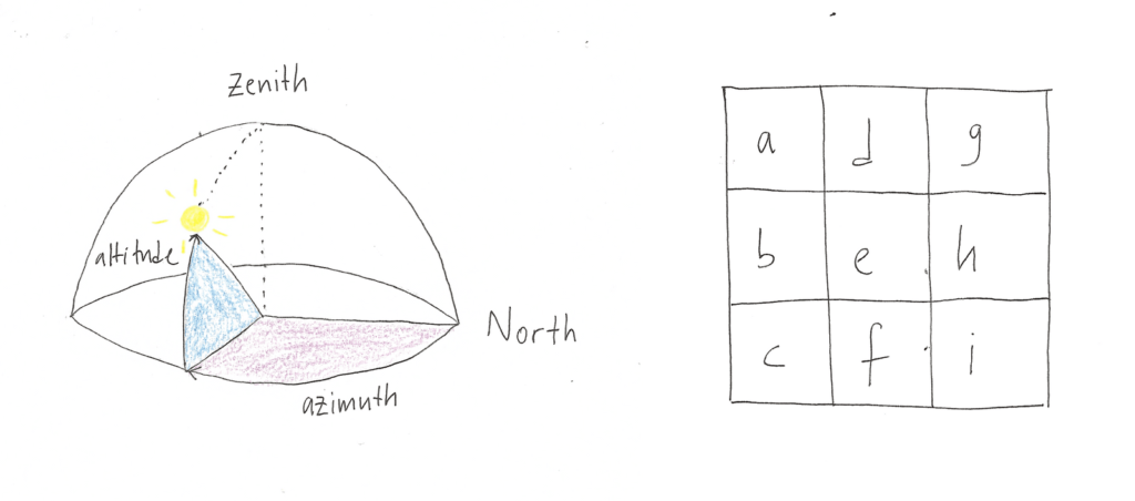
To calculate shaded relief from the DEM, we needed four values: The altitude angle, the azimuth angle, the slope, and the aspect.

The first two values are defined globally by us for the whole calculation:

• Altitude angle of the sun, which tells us how high the sun is standing on the sky surface. If it’s noon, the sun stands in zenith, meaning, the angle is 90°. If the sun sets, the angle is 0°. We used 45°, which you can think of as an afternoon sun – the shadows are not invisible (as they would be at noon), nor are they too long like at dawn.
• Azimuth angle of the sun. That’s like a compass direction. If the sun comes directly from the north, the azimuth angle is 0°; if it comes from the south, it’s 180°. In most hillshaded maps, you’ll see that the sun comes from northwest, so that hills are perceived as such and not as valleys. We went with the default value of 315°.

The slope and aspect for each pixel are calculated for each pixel, using the ratio of change in height of the eight neighboring pixels (so our so-called “kernel” is nine pixels big).

• Slope (steepness) of the terrain. As mentioned earlier, shaded relief doesn’t show the height of a location, but its steepness. That’s why we need to calculate the slope – is this pixel surrounded by pixels with the same grey value? Or is it surrounded on one side with pixels that have a lower value and on the other side with pixels with a higher value?
• Aspect of the terrain. That tells us in which direction the slope is facing.

These are the calculations:

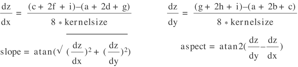
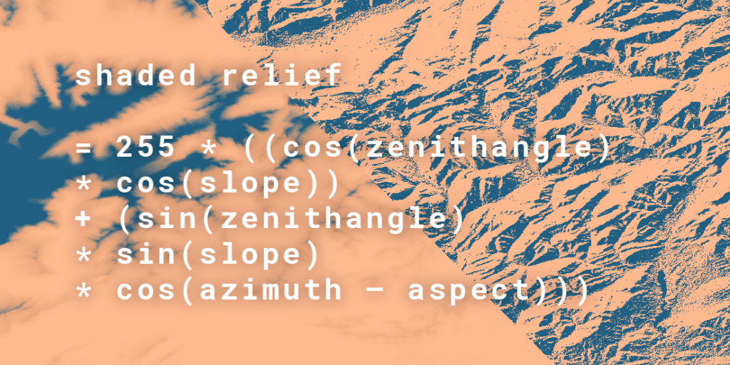
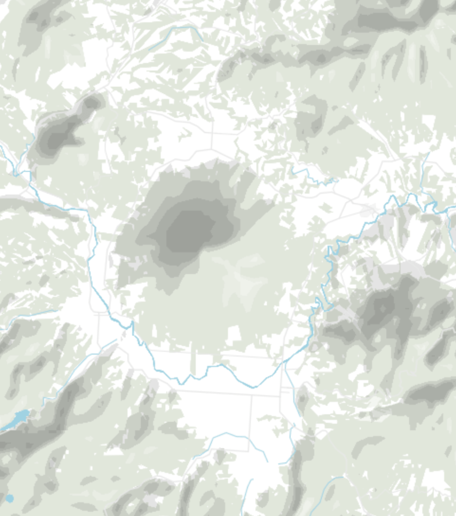
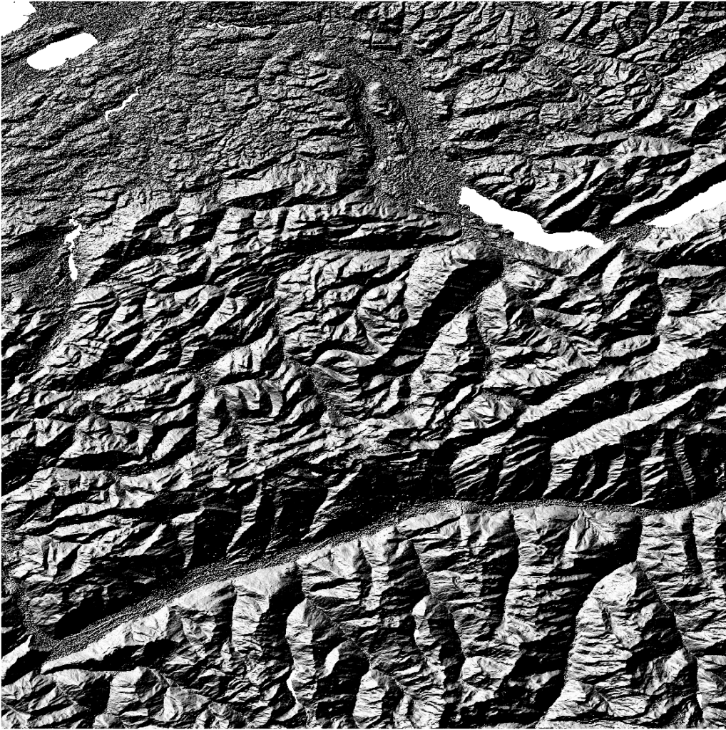
When the all the angles were obtained, we calculated the shaded relief value for pixel e with this algorithm:

shaded relief = 255 * ((cos(90 - altitude) * cos(slope)) 
    + (sin(90 - altitude) * sin(slope) * cos(azimuth – aspect)))

The result was a raster with shaded relief values from 0 to 255. Each pixel in this raster can again be shown as a grey tone, like in our DEM. But the hillshading values don’t give us information about the height, but is a combined value of altitude, azimuth, slope, and aspect:

• 

• 

A more detailed description of the algorithm can be found here.

GDAL has a nice, short command for calculating shaded relief for a DEM. It uses the default values for altitude (45°) and azimuth (315°):

gdal.DEMProcessing(target, source, 'hillshade', 
    options=[], azimuth=45, altitude=315)

3. Polygonoizing the raster

To create the vector tile layer, we had to extract polygons from the raster.

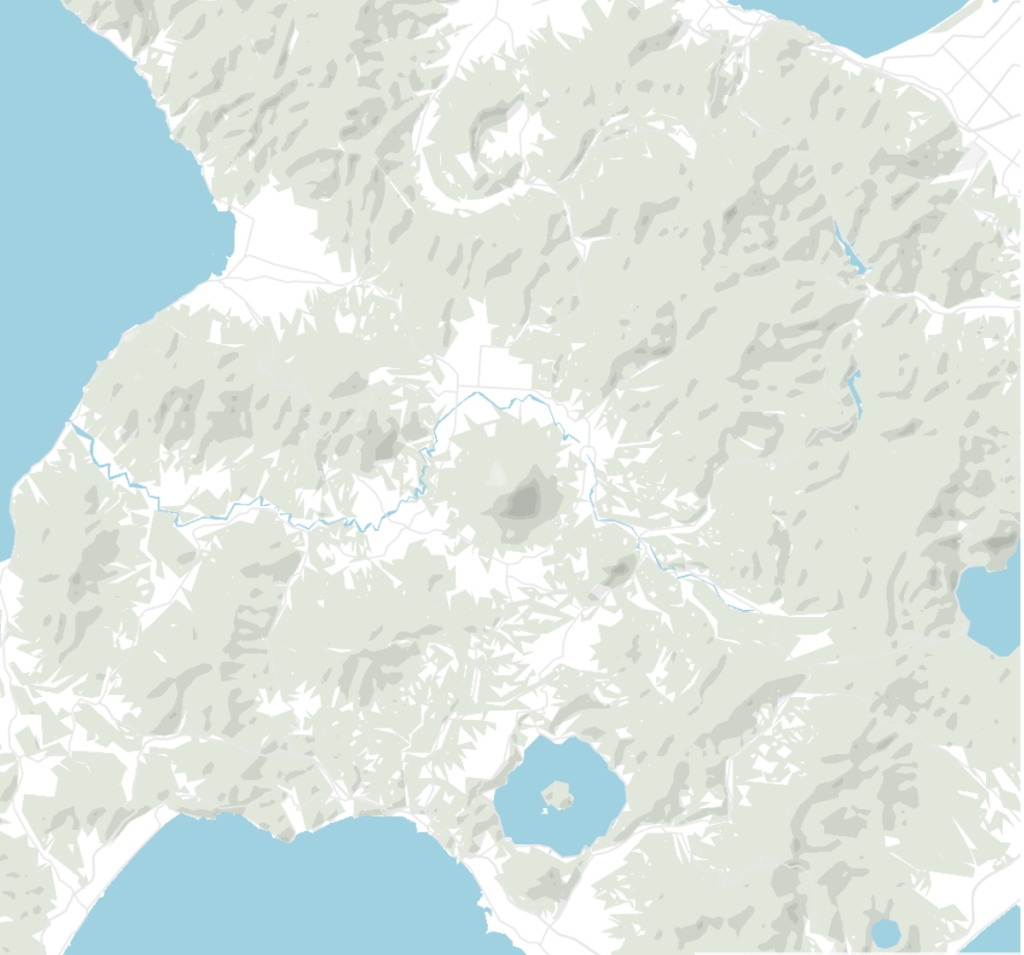
The polygons you see in the locator maps are divided into six classes, two classes for the brightest values for highlighting and four classes for the darker shades. Each class has an opacity and the steeper the hills are, the more polygons will overlay, the opacity adds up and the shade will get darker.

• 

• 

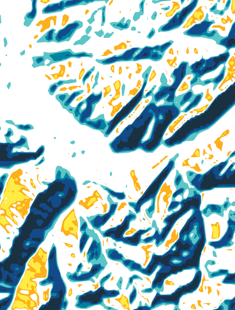
To group similar values from the shaded relief raster together to polygons, we used the GDAL command “contour”:

call(['gdal_contour', '-p', '-fl', 
    classification_value_min, classification_value_max, 
    source_raster, target_vector)

It extracts isoline polygons (lines with equal distance from each other), but the same concept can be applied to extract shaded relief polygons. Think about the classified grayscale values in the raster as areas with equal distances!

The polygons were exported directly to a PostGIS database and the vector tiles were generated.

Different zoom levels need different resolutions

All the fine details of the final shaded relief can’t be distinguished on lower zoom levels, so they don’t necessarily need the details of the raw data – and the embedded map would load too slowly with them, anyway. So for different zoom levels, we first decreased the resolution of the DEM, then did all the calculations, getting eight rasters for eight zoom levels.

To decrease the resolution for each zoom level, we used the GDAL command “Warp”:

gdal.Warp(target, source, 
    options = [xRes = res, yRes = res], 
    targetAlignedPixels = True)

We chose the resolution for each zoom level as a compromise of appearance and data volume:

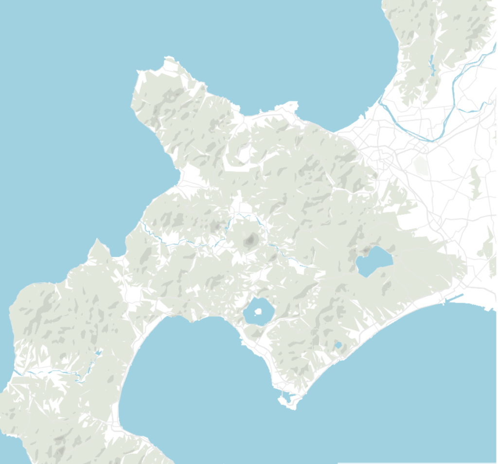
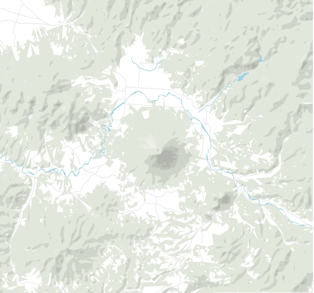
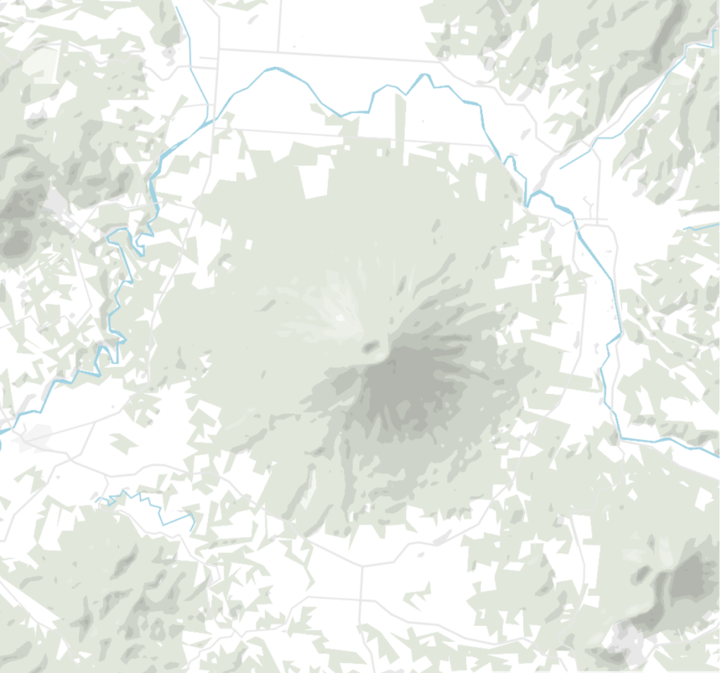
The resolution is 3000 m for zoom level 3 (meaning one pixel shows 3000m if you zoom out to see the whole world) and 100 m for zoom level 10.

Speeding up the calculations

The biggest challenge was to process (resample, calculate the shaded relief and vectorize) the 22192 TIFFs from NASA containing the height data.

A virtual raster saved us time and disk space. It “mosaiced” (combined) all the TIFFS, so that we could then access certain kernels or regions of it instead of going through TIFFS individually.

But even the virtual raster would get too big to hold the detailed shaded relief of the higher zoom levels in memory. The solution was to split up the virtual rasters in smaller chunks (10° stripes), which also had the benefit that the shaded relief could be run in parallel.

The polygonizing was the most time-consuming part of the processing. We sped it up by splitting the 10° areas in the raster into even smaller chunks (200px × 200px). We also ran the 10° areas in parallel processes. By doing this, we reduced the processing time from an estimated time of 6.5 weeks to around 26 hours. (In case you’re curious, we used an AMD Ryzen 7 1800X Eight-Core Processor with 8 cores per socket, 2 threads per core and 16 CPUs.)

---

We will continue to improve the layers for locator maps continuously. The next project is to add contour lines and add more detail to our green areas (like forests, deserts and agricultural areas). If you have any questions about this blog post, don’t hesitate to get in touch with me at anna@datawrapper.de or leave a comment below. Thanks for reading and stay tuned for more updates and improvements!

1. The ASTER is a Japanese space mission and it has acquired images of the earth since 2000. To create an elevation model from the images, they use a stereoscopic correlation.↩︎