How to match data with VLOOKUP in Excel & Google Sheets

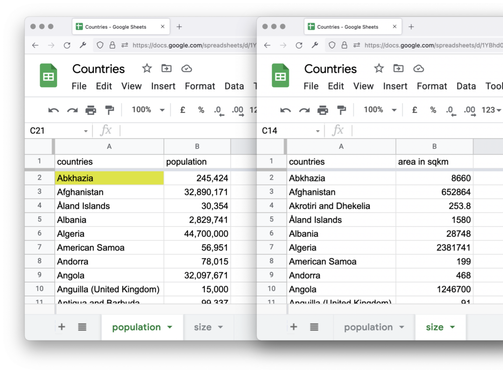
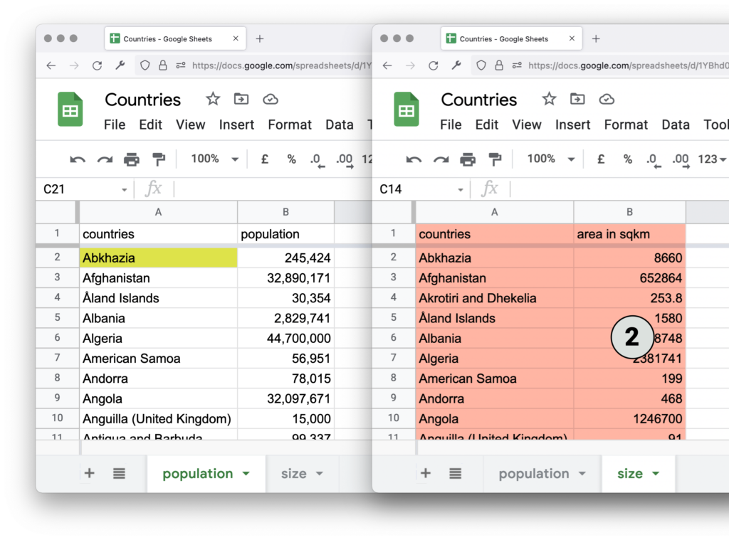
Let’s say you have two sheets in your spreadsheet:

• one showing a list of countries and their populations
• the other one showing a slightly different list of countries and their sizes in square kilometers

What’s the easiest way to join these two sheets into one table that shows the countries, their populations, and their areas? In Excel and Google Sheets, the answer is the formula =VLOOKUP(). I use it all the time to prepare data for my visualizations in Datawrapper. In this article, I explain how it works.

Here’s a video of everything you’ll learn in this article:

What is VLOOKUP?

VLOOKUP is short for “vertical lookup.” It lets you find cells based on other cells. For example, you can use it to ask Excel or Google Sheets: “Find Abkhazia in this column [in the size sheet] and return me its area from the column next to it.” (Abkhazia is a disputed territory on the Eastern coast of the Black Sea — yup, I also had no idea.)

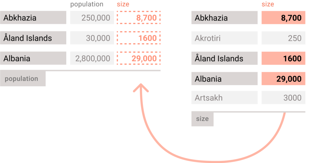
That’s especially helpful if you have different countries in your two sheets and can’t just copy the size column and paste it next to the population column.

How does VLOOKUP work?

The formula to use VLOOKUP is a bit tricky, so let’s go through it step by step.

First, create a column in which you want to do the lookup. We want to see the country sizes next to the population column, so I add a column called size next to it.

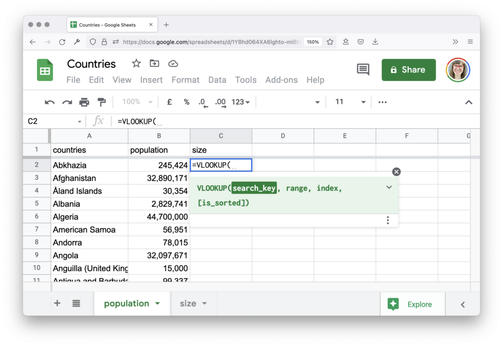
Now, type in =VLOOKUP(). This tells Excel or Google Sheets that you want to use this formula. It will ask you for four parameters:

• the search key (“Find Abkhazia…”)
• range (“…in this column…”)
• index (“…and return me its size from the column next to it.”)
• and the information if your columns are sorted alphabetically.

That’s a lot. Stay with me, we’ll go through it together.

VLOOKUP, step by step

Here’s an explanation of all four parameters that VLOOKUP needs.

First, the search key. It’s the country that exists in both of your sheets — the value you want to search by. Select it in your population sheet to search for it in the size sheet (so that you can then return the value in the column next to it).

In our population sheet, we select Abkhazia. It’s in A2, so the formula continues with =VLOOKUP(A2, ...).

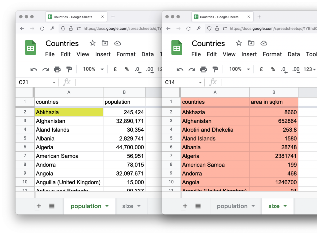
Next, the range. Here you tell Excel or Google Sheet where it should look for your search key. In our case, we want to search for Abkhazia in the size sheet, in the first column, A. But, ⚠️ attention: You need to include in the range not just the column where your search key is hidden, but also the column you want to return. So our range is not just the column with our countries, column A, but also the one with the size of the countries — columns A:B in the size sheet:

Now our formula looks like this: =VLOOKUP(A2, size!A:B, ...).

That was the hardest part.

The third parameter is the index. That one is easy: Count the columns in your range and tell Excel or Google Sheets which one it is you want to return the values of.

Our range has two columns: In the first column of the range, we look for the search key. Excel and Google Sheets know this one as “column 1.” Next to it is the column with the sizes. That’s “column 2.” Column 2 is the one we want to return the values of. So our index is… drumroll 🥁… 2.

Now our formula looks like this: =VLOOKUP(A2, size!A:B, 2, ...).

With the last parameter, you answer the question: “Is the column with countries sorted (most often alphabetically) or not?” with a TRUE or FALSE. You don’t need to add this fourth parameter — if you don’t, Excel or Google Sheets will pretend you answered: “Yep, it’s TRUE, they’re sorted.” I like to add a FALSE here for data like countries, just in case.

For our data, the formula

=VLOOKUP(search key, range, index, sorted?)

looks like this:

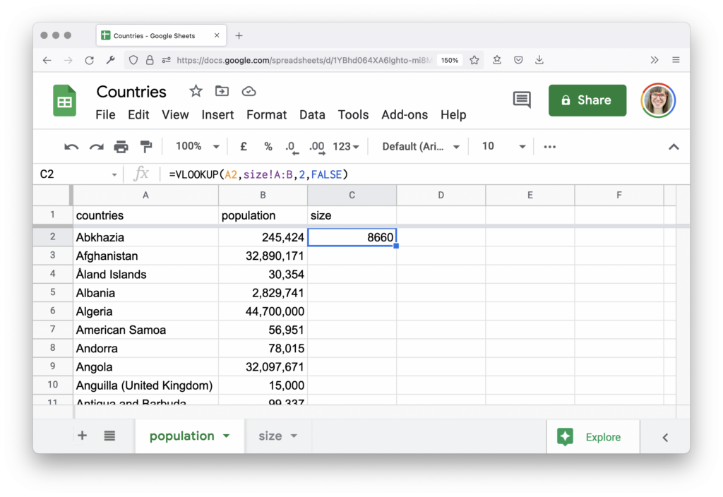
=VLOOKUP(A2, size!A:B, 2, FALSE)

If we type this into C2 (the first free cell next to Abkhazia) in the population sheet, we get what we wanted — the size of Abkhazia in square kilometers!

Applying VLOOKUP to the whole column

But we didn’t do all that work just for Abkhazia. It’s time to apply our formula to every country. To do so, select C2, then double-click on the little blue square in the lower right. This will apply the formula to all cells in column C that have a value in the column to their left:

How to select only part of the column as the range

It’s easiest to select whole columns for your range (A:B). If your formula’s range covers only part of the column in the second sheet (e.g. size!A2:B10) and you apply the formula to more than one cell, then the range increases (e.g. to size!A3:B11, then size!A4:B12 etc.).

If you want to avoid that, put a $ sign in front of the values you want to fix in place, like so: A$2:B$10.

Great — you just used the VLOOKUP formula to get a neat list of countries, their populations, and their sizes! That’s data you can now paste into Datawrapper to create a neat chart, map, or table. Here’s for example a scatterplot I created with this data inDatawrapper:

To try it out, click on Start creating on our website.

---

I hope this was helpful! If you need more help cleaning your data to prepare it for a charting tool like Datawrapper, visit our article “How to prepare your data for analysis and charting in Excel & Google Sheets”. And if you have any questions, please leave a comment or write to me at lisa@datawrapper.de.