How to split and extract text from data columns in Excel & Google Sheets

Sometimes, your data comes with several pieces of information in one column. Like a column with U.S. states in the format US-TX. Or a column with companies and the product they sell: Datawrapper (Software).

But say you want country (US) separate from state (TX) — for example, to create a Datawrapper choropleth map. Good thing there are easy ways to separate data points into two or more columns.

I’ll show two ways to create multiple new columns out of one old column. We’ll use Google Sheets — but the same tricks should work with LibreOffice Calc, Excel, or any other spreadsheet software.

The first method is the formula =SPLIT():

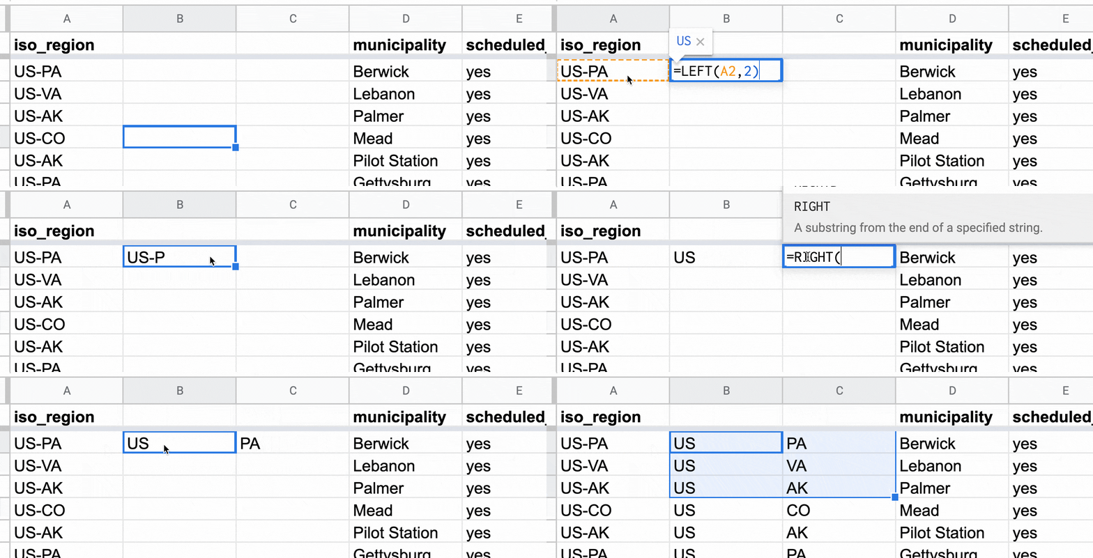
1. Create at least two new columns next to the column whose data you want to split. To do so, click on the header (A, B, C, etc.). Then click the little triangle and select “Insert 1 right.” Repeat to create a second empty column.
2. In the first empty column, write =SPLIT(B1,"-") (or =TEXTSPLIT(B1,"-") in Excel), with B1 being the cell you want to split and - the character you want the cell to split on. (If you see the error #REF! in your cell, you’ll need to create more columns.)
3. To apply the changes to the cells below, drag down the blue square in the bottom right of the selected cell(s). Double-click on the blue square to fill all remaining cells.

Sometimes you don’t have clear separator characters, but just want to extract the first or last characters of a cell. To do so, use the formulas =LEFT(B1,2), =RIGHT(B1,8), and =MID(B1,2,4):

1. Insert a new column. (Or two. Or three! As many as you need.)
2. In the new column(s), write
   =LEFT(B1,2) to extract the first 2 characters of the cell B1.
   =RIGHT(B1,8) to extract the last 8 characters of the cell B1.
   =MID(B1,4,2) to extract the 2 characters following the 4th character in B1.
   
3. To apply the changes to the cells below, drag down the blue square.

Pro tips

Pro tip 1: You can combine formulas to extract characters at all sorts of crazy positions. For example, the formula =LEN() gives back the number of characters in a cell. So =LEFT(A1,LEN(A1)-2) extracts the entire text in a cell except the last two characters. To separate the cell Datawrapper (Software) into the two cells Datawrapper and Software, you could use the formula =SPLIT(LEFT(A5,LEN(A5)-1),"(". This formula first removes the last bracket and then splits the remaining cell content on (.

Pro tip 2: Now that you learned to separate text, you can also bring it together again. To combine the column US from your cell A1 and TX from B1 with a hyphen, use ampersands and write =A1&"-"&B1.

Pro tip 3: You can extract content with LEFT(), RIGHT(), and MID() not just from text cells, but also from number and date cells. If you want to apply formulas like LEFT() to your dates, it helps to transform them into a text format first. To do so, use the formula =TEXT(A1, "MM/DD/YYYY"). Instead of MM/DD/YYYY, you can use any combination of these date codes and /, -, a space, etc. For example, =TEXT(A1, "dd-mmm-yyyy") will transform the date format 1st of November 2019 to a text cell with the content 01-Nov-2019.

Pro tip 4: If you have empty cells in your column, and you want them stay empty after using a function like LEFT(), you’ll need to check for these empty cells first. You can do so with the function ISBLANK(), combined with an IF function: =IF(ISBLANK(A1),"",LEFT(A1,3)).

---

I hope this was helpful! If you need more help cleaning your data to prepare it for a charting tool like Datawrapper, visit our article “How to prepare your data for analysis and charting in Excel & Google Sheets.” And if you have any questions, please leave a comment or write to me at lisa@datawrapper.de.